Building Vector Indices at Billion Scale
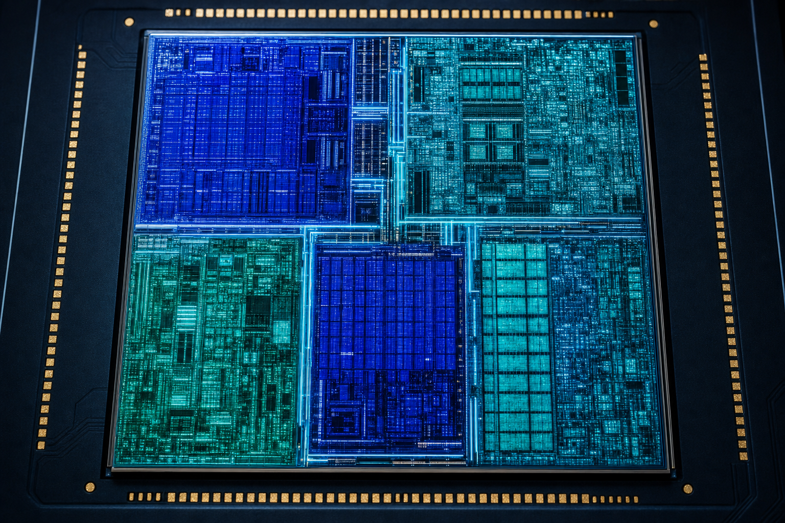
Valyu runs a petabyte-scale hybrid search index that spans the open web, financial filings, academic papers, clinical trials, patents, market data, and proprietary content. It holds billions of vectors today and grows continuously. At that scale, vector index construction is one of the many hard engineering problems we had to solve: it sets the rate at which new information can enter the index.
Of every operation in a vector index's lifetime, building the graph that queries route through is the most expensive. At our scale, the algorithms and execution models that work for smaller indexes break.
We rebuilt the initialisation path of our vector index to reach these scales. A build that took 80 minutes at 10M vectors now completes in about 25 minutes for 100M vectors on a single GPU. The same pipeline parallelises across GPUs to reach billions.
Graph walks are the wrong default for index initialisation at this scale. With the right hardware and workload shape, exact sweeps beat them. Below, we work through why, and how the same exact primitive moves from CPU to GPU as the corpus grows.
The two phases of initialisation
Vector index initialisation has two distinct phases that do different work.
The first builds the head graph: a navigable graph over centroids that subsequent queries route through. Recursive bisection splits the corpus into balanced buckets and produces leaf centroids. A small relative-neighbourhood graph is built over those centroids. A handful of entry seeds are chosen for query-time traversal. The output is the structure the index uses to answer queries.
The second phase is vector assignment. Every input vector finds its K-nearest centroids in Hamming distance and is appended to each of those K posting lists. A vector lives in K posting lists rather than one because that's what gives the index its recall safety margin: when a query's true-nearest centroid is not the first one probed, the right vectors still surface from one of the others.
Diagram: index architecture overview, showing head graph build and vector assignment as the two distinct phases.
The two phases have different cost profiles. We instrumented the original CPU implementation at 1M and 10M:
| Phase | 1M | 10M |
| Bisection (head graph build) | 23.8 s (38%) | 3.6 min (6%) |
| Vector assignment | 37.9 s (60%) | 56.6 min (88%) |
| Relative-neighbourhood graph + entry seeds + posting writes | 1.1 s (2%) | 4.1 min (6%) |
| Total build_index | 62.8 s | 64.3 min |
Assignment dominates, and it dominates more as N grows. The reason is structural: assignment runs N x C Hamming top-K searches, while bisection runs closer to O(N log N) work. Both phases needed work.
Two facts shape our approach. The first is the centroid count C, which under our formula scales linearly with the corpus:
That C ~ N is a deliberate operating point, traded against recall and posting-size variance. It's also what makes assignment quadratic in N at large scale: assignment is N x C, and C is itself proportional to N.
The second fact is that the distance primitive is cheap. Our search system uses 512-bit binary vectors, so the distance between two of them is Hamming distance, i.e. the popcount (number of set bits) of the XOR:
Diagram: bit-level XOR and popcount.
On modern Intel x86 CPUs with AVX-512 and VPOPCNTDQ, a 512-bit Hamming distance takes about 5 nanoseconds: one ZMM register, one XOR, one popcount, a horizontal sum. Floating-point dot products, by contrast, are an order of magnitude more expensive and don't pin cleanly into registers in the same way.
The two phases need different treatment. The head graph is a cache problem; assignment is a primitive-choice problem. We tackle them in order.
Building the head graph
Bisection looks small in the 10M instrumentation (6% of build) but explodes at 100M. The cause is cache pressure, not algorithmic complexity.
The original head graph build is a global recursive bisection. Take the full corpus of N vectors, split it in two using k-means, recurse into each half, and continue splitting until each leaf bucket holds about target_posting_size vectors and produces a centroid. Around those centroids a small relative-neighbourhood graph is built and entry seeds are selected, but those steps are trivial at the centroid counts we work with: sub-second even at 30M. Bisection is the only part of the head graph build that scales with N.
The cost during recursion is what kills it. Every level of the tree touches every vector in the corpus: level 0 splits N vectors; level 1 splits each half independently but still touches N in total; level 2 touches N; and so on. At 100M with C ~= 400K, the recursion is log2(400K) ~= 19 levels deep - about 1.9 billion vector touches, not counting per-pass overhead. The depth itself is fine. The problem is cache: early-level working sets are far larger than L3, so every pass at the upper levels runs cache-cold and bisection ends up cache-pressured superlinear.
The structural fix is to stop touching the full corpus at every level. Sample 2M vectors, train a coarse routing tree on them, route every vector in the full corpus through that tree once, then bisect each bucket independently down to leaf-level centroids. The corpus is touched once, in the routing pass. Everything after is bucket-local, and the buckets fit comfortably in cache.
Diagram: bucket-local versus global bisection.
Bisection wall time goes from cache-pressured superlinear to close to linear, with the scaling exponent dropping from 1.13 to 1.09 between 1M and 30M:
| N | Global recursive | Bucket-local | Speedup |
| 1M | 13.17 s | 2.69 s | 4.9x |
| 10M | 171.68 s | 33.74 s | 5.1x |
| 30M | 617.86 s | 108.72 s | 5.7x |
Memory layout matters at this scale too. A traditional build path that holds buffered vectors live in memory exhausts a 32 GB machine around 16M vectors. The streaming approach is a fixed-stride binary slab on disk with 72 bytes per record (a u32 vector id, a u32 doc id, and the 64-byte binary vector) read through in large contiguous chunks. RSS tracks the working set, not the full corpus, and the build runs on cheaper hardware regardless of corpus size. The slab also happens to be the right shape for feeding a GPU, but more on that later.
With bucket-local bisection and the slab in place, the head graph build at 30M is about 110 seconds. At 100M it rises to 7 minutes. The head graph phase is effectively solved on CPU; assignment now dominates everything else.
Vector assignment on CPU: when brute force beats graph walk
When a single comparison costs 5 ns, an exact sweep over thousands of centroids can be cheaper than any algorithm that tries to be clever about which centroids to visit.
Vector assignment runs once per input vector: find the K-nearest centroids in Hamming distance. The original implementation used the same graph walk the index uses at query time.
At query time, this is the correct approach. Queries arrive one at a time, latency matters, and skipping most of the centroid set is the point of having a graph. At assignment time the workload shape inverts. Millions of vectors are already available; throughput matters; the centroid set is reused for every query; and an exact top-K answer is both achievable and slightly better than the graph walk approximation.
The right primitive falls out of the costs:
Brute force does many cheap operations. Graph walk does fewer expensive ones. Both terms scale with C, but not the same way: brute force is proportional to C with a constant per-comparison floor, while graph walk's per-visit cost itself grows with C as the centroid array falls out of cache and neighbour-pointer chasing runs cache-cold.
The measured asymmetry is stark. Graph-walk per-search at 1M (1K centroids) was 35 microseconds. At 10M it was 390 microseconds - over 10x slower for a 10x larger corpus. The crossover where brute force wins is the point at which C x 5 ns is less than V x per-hop-cost, and because the per-hop cost grows with C, the crossover comes well below the centroid counts a real corpus produces.
At 10M with K=4, the centroid array is 40K x 64 bytes ~= 2.5 MB, comfortably L2-resident. A brute-force kernel that flat-sweeps all centroids runs at about 5 ns per Hamming including loads and heap maintenance. Replacing the graph walk with a flat O(C) SIMD sweep drops per-search cost by about 4x and drops total assignment from 56.6 minutes to 12.8 minutes.
Animation: graph walk versus brute force traversal.
Brute force is also exact. It returns the true K-nearest set, not the graph walk approximation. The assignment step itself can only become more accurate, because it now returns the exact K-nearest centroids. In our held-out query evaluation, end-to-end vector recall improved by a small but measurable margin.
Tiling and pinning
The first version of brute force leaves per-Hamming cost around 10 ns, about 80% of which is bookkeeping, not arithmetic operations. Two layered optimisations reduce this.
The first is query tiling. Process 64 queries against the same centroid stripe per tile, instead of one query at a time. Each centroid is loaded once per tile rather than once per query. At 40K centroids and 10M queries, that is a 64x reduction in per-centroid bookkeeping, with the centroid staying hot in registers across the inner loop.
Animation: query tiling, one centroid held while 64 queries flash.
The second is pinned-centroid SIMD. A naive Hamming routine does a runtime feature-detect per call and reloads the centroid inside the SIMD body. Both are fine when called once; both burn cycles when called 77 billion times. A batched primitive that feature-detects once per call, loads the centroid into a ZMM register, and holds it pinned across the entire query batch brings per-Hamming cost from 10 ns to 6.9 ns.
These two changes are scale-dependent. At 1M, the centroid array is 64 KB which fits entirely in L1 cache and the per-tile setup actually shows up as a 5% regression. At 10M, the array is 2.5 MB and L2-resident, and tiling significantly improves on the L2 traffic.
The CPU assignment optimisations at 10M, end to end:
| Phase | Graph walk (baseline) | + Brute force | + Tile + Pin | Total speedup |
| Vector assignment | 56.6 min | 12.8 min | 8.84 min | 6.4x |
| Build_index total | 64.3 min | 16.8 min | 12.75 min | 5.0x |
Vector assignment on GPU: killing the quadratic
Scaling assignment to 100M shows the limit of the CPU path. Under the centroid-count formula:
At 100M, that is 40 trillion Hamming comparisons. Quadratic in N. The CPU brute-force kernel runs them at its theoretical floor, but the absolute volume is what kills it.
A single-threaded AVX-512 kernel runs at 0.32 GH/s per core. 44 SMT threads on an x86 machine aggregate 7.25 GH/s - a 22x scale-up, not 44x, characteristic of AVX-512 shared 512-bit execution units and turbo throttling under sustained load. Projected forward, a 100M CPU build is about 10 hours, dominated entirely by assignment.
The remaining quadratic term needs different hardware.
Assignment is a textbook GPU workload. The batch is huge. The centroid table is reused across millions of queries. The inputs are fixed-width binary. Distance calculations are independent. There is no per-query latency requirement, and the output is a top-K, small per query.
We wrote a simple custom kernel: one thread per query, per-thread top-K maintained in registers via insertion sort and centroids read from GPU memory. On L4 GPU at 30M x 120K, it takes about 10.4 seconds for the kernel itself, plus a few seconds of host-side overhead. The kernel scales linearly with centroid count, as expected for a flat sweep. It has the same semantics as the CPU brute force and is validated against the CPU result set on every test, confirming that GPU assignment is purely an indexing speed-up and does not change the underlying graph structure.
At matched workload shape (30M vectors, 120K centroids, 64-byte binary vectors, K=4), measured median of five:
| Platform | Wall time | Throughput | Relative |
| L4 GPU | 14.73 s | 61.1 GH/s | 1x |
| 44-thread Intel x86 CPU, AVX-512 | 124.16 s | 7.25 GH/s | 8.4x slower |
The kernel runs at about 488 billion 64-bit popcounts per second. Profiling puts it at 93% of compute throughput on the pipeline it is bottlenecked on: the GPU MIO unit, where the CUDA popcount intrinsic popcll shares cycles with branches and shared-memory ops. The L2 hit rate is 100%, so the centroid table stays in cache the whole time. The kernel is not memory-bound; it is pegged on the only pipe that can issue its hot instruction.
With the kernel at its compute ceiling, data movement and orchestration become the next constraint. The slab from the head graph build now earns its keep on a second front: large contiguous chunks of fixed-stride records load from disk into CPU memory the GPU can read directly, transfer asynchronously to GPU memory, run through the kernel, return as compact top-K results, and get appended to the posting lists on the CPU. Each chunk stages overlap with the next chunk stages. While the GPU runs the kernel on one chunk, the CPU prepares the next and writes results from the chunk before that. In steady state, disk reads, PCIe transfers, GPU compute, and CPU posting writes all run concurrently.
Animation: pipeline overlap in steady state.
The 30M GPU build that takes 379 seconds end-to-end includes only about 40 seconds of actual kernel time; everything else is the data path like reading records, packing them on the CPU, and transferring to and from the GPU.
100M end to end
At 100M, under the centroid-count formula (K=4, target posting size 1000), the centroid set is about 400K and the assignment work is about 40 trillion Hamming comparisons. Phase-by-phase:
| Phase | Original CPU path | CPU + bucket-local | GPU path |
| Bisection (head graph) | ~hours (superlinear) | ~6-8 min | ~6-8 min |
| Vector assignment | ~9-10 hr | ~9-10 hr | ~10-15 min |
| Posting writes | ~5 min | ~5 min | ~5 min |
| Data staging | n/a | n/a | ~2-3 min |
| Total | ~10+ hr | ~10 hr | ~20-30 min |
After the GPU pivot, the bottleneck shifts. Before, assignment dominated everything - 90%+ of build time at 30M and 100M. After, bisection and posting writes are back on par with assignment. That is the right outcome. The largest phase has been moved onto hardware suited for dense batched Hamming top-K, and what remains is distributed across phases that will not benefit from the same hardware swap. The next round of work goes to those phases.
Diagram: bottleneck shift before and after GPU.
Why not FAISS or HNSW?
Stepping back, the obvious question: why not just reach for an existing library like FAISS, cuVS, or hnswlib? Two reasons.
First, binary vectors are second-class in most of them. These libraries are tuned around float vectors and L2 / inner-product distance; their fastest kernels assume floating-point dot products, not VPOPCNTDQ. The 5 ns Hamming primitive that drives every decision in this post only exists because the distance primitive is this cheap on our representation.
Second, our index structure is not HNSW or IVF-PQ. The head graph is a navigable graph over centroids, but the posting lists hanging off each centroid hold vectors with K-way replication for recall safety, and the whole layout is designed for streamed continuous updates: new vectors route through the head graph and append to K posting lists without rebuilding it. FAISS GPU is built around one-shot batched construction with the corpus resident in GPU memory; hnswlib incremental build does not share the replication semantics. Adopting either off-the-shelf would have meant changing both the index format we serve queries against and the update model we depend on.
When the primitive changes
The shape of the problem changed as the index scaled. Graph walk is a good query-time primitive because it avoids most of the centroid set under tight latency. During initialisation, the workload is different: vectors arrive in bulk, centroids are reused heavily, and binary Hamming comparisons are cheap enough that exact sweeps become competitive.
That is why the implementation moved from graph walk, to CPU SIMD brute force, to GPU brute force. The idea did not get more complex; the execution model became better matched to the work.
The GPU kernel now sits at its compute ceiling on the popcount path, so the next step will not be a tweak. The hardware path is the int1 BMMA tensor cores, a separate physical pipeline at roughly an order of magnitude more throughput alongside GPU parallisation on newer hardware like A100 and H100s. The algorithmic path is a graph-narrowed candidate set followed by brute-force reranking, the two-stage shape we expect for larger graphs.
Brute force does not always win. The useful habit is to re-evaluate the primitive whenever the scale changes. The abstraction that is right for one part of the system can be wrong for another. In this case, the fastest path came from treating index construction as a dense batched compute problem rather than as a sequence of approximate searches.
Want to try Valyu yourself?
Build with the same Search and DeepResearch APIs at platform.valyu.ai.
More from the blog


Valyu Add
Join 12,000+ professionals and knowledge workers.
Valyu Add is a free weekly research briefing for builders, investors and operators. Every issue is sourced, cited and verified with Valyu DeepResearch.